Creating Infinite Bad Guy
Infinite Bad Guy brings together thousands of YouTube covers of Bad Guy by Billie Eilish into an experience that lets the viewer jump from one cover to another, always in-time and without skipping a beat, guided by similarities and differences in each performance.
Google Creative Lab invited IYOIYO to contribute an audio and video analysis pipeline, including a novel music alignment algorithm that matches the beats of cover songs to the original song. This work was led by Kyle McDonald and included a small team of developers and data labelers.
Crowdsourced music videos have a long history, with the first wave responding to the rise of social media around 2009–2010 with 日々の音色 (Hibi no neiro) by SOUR with Masashi Kawamura, More is Less by C-mon and Kypski with Moniker, and Ain’t No Grave by Johnny Cash with Chris Milk. In 2010 creative crowdsourcing was top-down, with precise directions guiding the crowd to form a cohesive whole. But “Infinite Bad Guy” has more in common with artist Molly Soda’s hand-aligned covers in “Me Singing Stay by Rihanna” (2018). In 2020 crowdsourcing is bottom-up, with machine learning finding our commonalities at a massive scale.
The Task
After some early experiments, we picked three deliverables that could be used to build the experience. Given a cover video, we would:
- Estimate the per-beat alignment between the cover and the original.
- Visually classify the video.
- Identify the most visually similar videos.
On this project IYOIYO focused on research and development. Other teams from Google Creative Lab implemented the production infrastructure and frontend, with IYOIYO advising on integration of our pipeline that outputs an analysis file for each track.
Audio Alignment
Every cover song is unique. But from an audio analysis perspective there are a few broad categories with specific alignment challenges. Ordered from “easiest” to “most difficult”:
- Copies of the original. This includes dance covers, workout routines, lyric videos and other visual covers.
- Covers with digital instrumental backing tracks. There are only a handful of popular instrumental and karaoke covers of Bad Guy, and these are often used as a backing track for a family of string musicians, violinists, or vocal covers.
- Full-band covers, which are typically not recorded against a click track and can vary significantly in song structure. Like this Irish Reggae Trio, or this metal cover (though metal covers usually have impeccable timing).
- Remixes and parodies that reference a very short portion of the original track, or drastically transform the original track. This includes multi-million-view parodies like Gabe The Dog and Sampling with Thanos, but also the Tiësto remix.
- Purely acoustic solo covers, which have similar challenges to full-band covers but fewer musical indicators useful for automated analysis. For example these covers on clarinet, on guitar in a bathtub in a monkey onesie, or any of the many ukulele covers.
Around 1 out of 4 covers belong to the first two categories, and they can be very accurately aligned using a simple technique because there is only one important number: the offset between the original track and the copy (or instrumental backing track). This offset can be determined by checking the cosine similarity at different offsets: this means taking the spectrogram (a visual “signature” of the sound) of the cover and the spectrogram original, and sliding one past the other until they line up best.
For the remaining three categories¹ — full-band covers, remixes, and solo acoustic covers — we need a different approach. The tempo of these covers can vary significantly from the original, and can vary internally as well. We first tried two approaches that were not robust enough: dynamic time warping and chord recognition.
Dynamic Time Warping and Chord Recognition
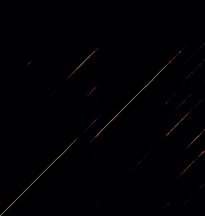
Dynamic time warping (DTW) is the go-to algorithm for aligning two sequences that vary in their rate, duration, or offset (see also Serra et al from 2008, and Yesiler et al 2019). This is what it looks like using DTW to align audio features between a cover and the original:
The thin white line can be read as starting at the very top left corner. It briefly goes straight down, meaning that there is no corresponding section between the original (on the Y axis) and the cover (on the X axis). This is because the original has a brief spoken-word section, but many covers begin on the first beat. The line then continues along a 45 degree diagonal, along the “valley” or lowest-cost path through the distance matrix. The 45 degree diagonal indicates that the two songs are at the same tempo.
Dynamic time warping has two major issues that made it less than ideal. First, DTW cannot handle repetition. If a cover repeats a section from the original, the DTW cannot “backtrack”. If we run DTW the other way, aligning the original to the cover instead of vice versa, then “repetition” appears as “deletion”. DTW can handle this, but if there is both deletion and repetition in a cover then we are stuck (and both are common).
DTW can also be very computationally intensive, but even after optimizing it we ran into a bigger issue: what features to use when determining “distance” between two moments? Some cover song identification algorithms use chords; we could also try to extract the melodic line, or some other audio features. Tuning these features can work very well for one set of covers, then completely fail for other covers. For example, the raw spectrogram works wonderfully for near-copies, but fails on covers in different keys, or covers without a similar beat.
Because existing cover song alignment and identification algorithms rely so heavily on chord recognition, we tried it out next. In the best cases, we would see a sequence of chords as below: a long period of no music, then Amin, Dmin7, E7, and then repetition (with X indicating unknown chords).
Although this is one of the 5% of covers that are not in Gmin, we can easily transpose this to the original key of Gmin and then identify the corresponding section changes. But this technique fails for a few important reasons. The biggest reason becomes obvious when we look at the chord recognition results for the original song.
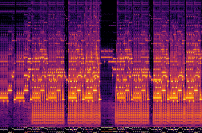
The original is often harmonically rich, but most of the chords are only implied by the bass or hinted at by the vocals, and rarely completely voiced. Very many of the covers emulate this stylistic choice, or sometimes they are performed on monophonic instruments. Chord recognition systems are not designed to deal with any of this, so they fail miserably.
A New Approach
The deeper we got into the alignment task, we realized we had two major challenges:
- Determining the accuracy of the alignment algorithm efficiently. Heuristics give fast results, and can be tuned easily, but without ground truth labels each of those results must be hand-checked.
- Handling the more than 1 in 7 covers that repeat a section, or the many other covers where DTW or offset alignment would fail.
We switched from hand-engineered heuristics to treating alignment as a machine learning task. We built a dataset of aligned covers and trained a recurrent neural network (RNN) to solve the beat classification task. The heuristic solutions helped bootstrap this by producing a set of sometimes-accurate labels. This turned the dataset building into a validation job instead of a labeling job.
Dataset Building

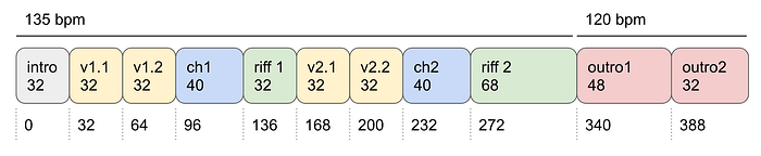
We built an interface for very quickly validating section-change labels as either correct or incorrect: clicking or tabbing through the labels instantly played that section, then the cover was marked as good, bad, or not a cover (usually an unrelated song with a similar name). Each section had a code name, like “ws” for the verse beginning “White shirt now red…” and “br” for the verse beginning “Bruises on both my knees…”². We averaged around 100 validations per hour, and collected over 5000 validated results. This helped us learn that the heuristic algorithms were only correct around half the time. The validated predictions gave us a starting point for training the RNN.
We also created section-change labels for 1000 covers in Audacity. This takes a lot longer, at only 30 per hour, but after the first few spectrograms it’s possible to drop labels without listening to much: it’s easy to visually identifying many section changes.

While the offset alignment and DTW provide a dense set of labels (with section-change labels validated as a proxy), manual section-change labels had to be converted to dense labels. We used some heuristics, like knowledge about the song structure and tempo consistency, to estimate interpolated dense markers. Only a few sections significantly challenge these heuristics, like the few pauses throughout the song (“duh”) which are sometimes extended with a fermata.

Recurrent Neural Network Alignment
With a set of thousands of manually labeled and automatically labeled and validated cover song alignments, we were able to train an RNN. The input to the RNN is an nxm matrix: n cover beats, and m audio features. The output is an nxk matrix: n cover beats, with each beat providing a probability distribution across k original beats. We treated “Bad Guy” as having k=420 beats:
The RNN was implemented in Keras. An architecture search yielded a very simple network as optimal: a single bidirectional LSTM layer of width 1024, followed by batch normalization, very high dropout (0.8), and a dense layer with softmax output. Other RNN architectures with additional noise, different dropout, more or less layers, more or less units, all gave a similar validation accuracy around 80% which suggests the architecture was not the primary accuracy bottleneck. During training the input looks like this:
And after training the output looks like this:
The RNN mostly learns about temporal consistency: covers do not often jump from one section to the next, or rearrange beats (except for this cover that swaps the 2 and 4 beats). But to provide an extra guarantee of temporal consistency we apply a diagonal median filter before taking the highest-probability prediction.
The final pipeline starts with the offset-based alignment algorithm, and if it is a good match we use that solution. Otherwise we fall back to RNN alignment for the harder covers. RNN alignment starts with beat tracking³, which provides timestamps for all the beats in a track. After beat tracking, we extract a constant-Q transform spectrogram and chroma features from each cover beat chunk and use the RNN to make make original beat predictions. Our validation set consisted of 100 covers that represented the content that we wanted to prioritize: especially acoustic and vocal covers rather than electronic remixes and short parodies. Below, the orange line represents the true alignment and the blue represents the predicted alignment.
Most covers could be solved by the offset alignment algorithm (white background) though it sometimes resulted in mislabeling of brief repetitions, or incorrect offsets for a very repetitive cover. The RNN alignment (gray background) goes wild when predicting beats before or after the cover (like a non-cover musical intro/outro), but these predictions are also typically very low-confidence and can be thresholded and discarded.
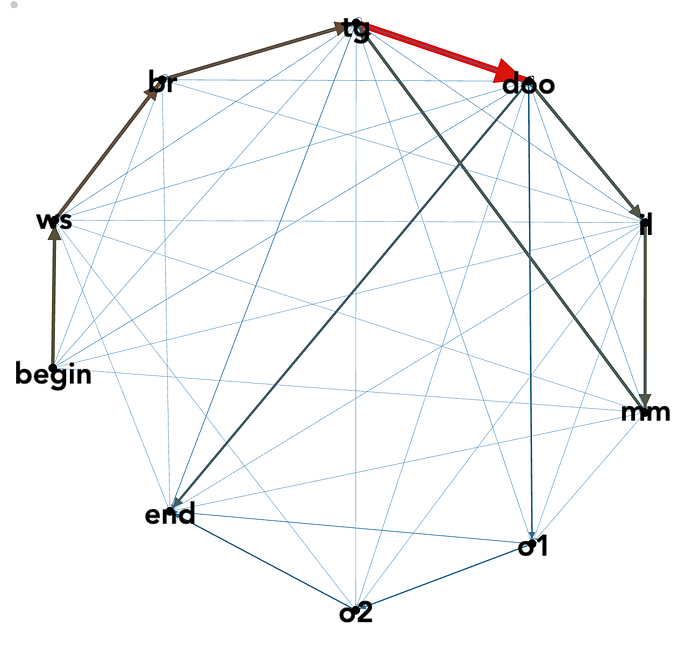
For additional robustness when handling covers with a different structure than the original, we built a transition matrix describing the frequency of section changes in different covers. Then we used these probabilities to create augmented versions of existing covers: ending them early, skipping the intro, repeating a commonly-repeated section, etc. This was combined with other kinds of audio augmentation including noise, random spectral equalization, and small beat timing offsets.
The final RNN yields around 83% validation accuracy in identifying the original beat for a given cover beat. Around 60% of the covers have more than 90% of the beats identified correctly. A major constraint on the system is that librosa’s beat tracker only tracks 88% of beats to better than 1/16th note accuracy (around ±110ms). This means that 12% of the beats from the beat tracker may not be categorized correctly because the boundaries of the beat are inaccurate.
Wondering if this accuracy might be improved with better features, we tried YAMNet embeddings and contrastive predictive coding embeddings (CPC). YAMNet was trained on the very large AudioSet corpus and accurately predicts sound categories across more than 500 classes, but the embedding was no more accurate than our chroma + CQT baseline. Similarly, CPC trained on 15k unlabeled covers gave us no more accuracy. We also tried harmonic pitch class profiles (used in some cover identification work), and harmonic CQT, which both performed similarly to the baseline. This suggests the accuracy limitation may be in the dataset or beat tracking. One change that did help slightly was enhanced chroma with harmonic separation and median filtering.
One of the hardest challenges that is not handled by our architecture is deciding whether a specific portion of a song is a cover or not. Someone playing a kazoo could be part of a channel’s intro music, or it could be a kazoo cover of “Bad Guy”, or it could be a kazoo mashup of “Bad Guy” and “Plants vs Zombies” and we are listening to the “Plants vs Zombies” part. The only way to know is by analyzing the track as a whole, and this is nuance that a bidirectional RNN may not always capture.
For future work we would explore:
- Newer unsupervised algorithms (including newer versions of CPC).
- Replacing beat tracking with fixed-sized 100ms chunks.
- Label smoothing to afford more continuous timing predictions.
Visual Analysis
Image classification and video classification was more obviously favorable for a machine learning approach from the beginning. In the end, most of our work on visual analysis was replaced by existing tools at Google. But the process is worth sharing as a study in what it looks like to create this kind of system from scratch, and in what kind of videos exist across YouTube.
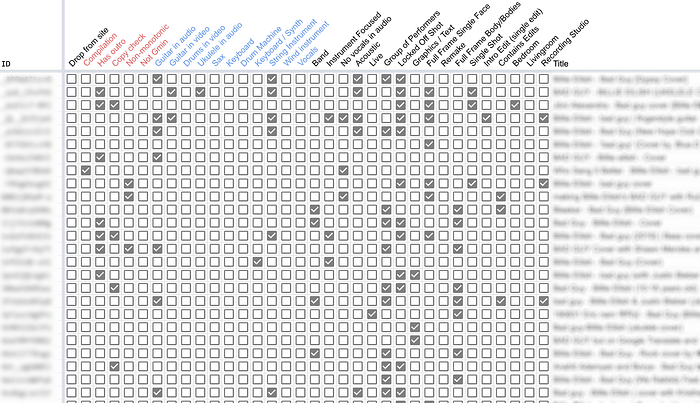
We started by building an ontology and small dataset describing 200 cover videos. A massive grid of checkboxes in a shared spreadsheet.
Our first ontology was based on identifying a few major categories:
- There are a few shot-for-shot remakes and aesthetically inspired remakes. This metal cover, this Indonesian cover, frat guy, the Otomatone cover, and many composited versions. These are some of the most carefully crafted cover videos, but also the hardest to automatically distinguish from re-uploads of the original video. We wanted to make sure we caught as many of these as possible.
- Dance videos. We initially trained a network to identify these, and discussed using pose estimation as an input to the classifier, but ultimately found that Google had a better internal dance detection algorithm.
- Videos with still graphics or lyrics combined with a karaoke track, or screen recordings of digital audio workstations for music creation tutorials. We identified these to help us prioritize covers over tools and tutorials.
For all the other videos we labeled shot framing (close/medium/wide) and instruments (band/strings/keys/wind/drums/pads). Our first pass of 200 videos was enough to help familiarize us with the diversity of the cover videos and validate our ontology, but ticking boxes in a spreadsheet is very slow and couldn’t get us to the scale of data we needed for training a classifier. So we built another labeling tool based on visual similarity⁴.
Labeling
To label a larger number of videos more efficiently, we built a tool that groups videos based on visual similarity and provides a set of button to tag each video. Videos are presented as a series of nine evenly spaced frames in a photo roll. The video at top is used as a reference video, and the next 10 videos are the most visually similar videos. After finishing one page, another reference video is pulled from the queue of unlabeled videos. When a video has been tagged, it does not reappear later in any list of visually similar videos. We used an iPad Pro to quickly label thousands of videos this way, at a rate of around 500 videos per hour.

We built the video labeling interface in less than 100 lines of Python using Jupyter Lab with ipywidgets. The most important part of the interface is the visual similarity algorithm.
Visual Similarity
To measure similarity between videos, we started by feeding each frame of each video through the MobileNetV2 image classification network. This gave us a matrix of nxm values for each video where n is the number of frames and m is the number of output features from the network⁵. For example, a three-minute video at 30fps will yield 5400 frames x 1280 features. This matrix of values cannot be directly compared between two videos because n varies. We tried a few approaches to getting a “summary” of this matrix: taking the mean value across all features over time, the max value, the standard deviation, or some combination of these. These worked for locked-off videos, but none of these approaches captured similarity for the videos that had a lot of edits and camera movement (like remakes). So we engineered a custom feature vector that balanced all the different aspects of “similarity” we wanted to captured.
- Select a small k evenly spaced feature vectors from the original nxm matrix. This captures a “summary” of the shots in a video, and is most helpful for identifying remakes and copies of the original.
- Take the mean of the absolute value of the intra-frame differences for all frames. We call this “activity” and it captures the presence of short-timescale changes like camera moves and cuts.
- Take the max of the absolute value of the intra-frame differences for only the selected k frames. We call this “diversity” and it describes roughly how many kinds of shots there are throughout the video, and what those shots capture.
The code looks like this:
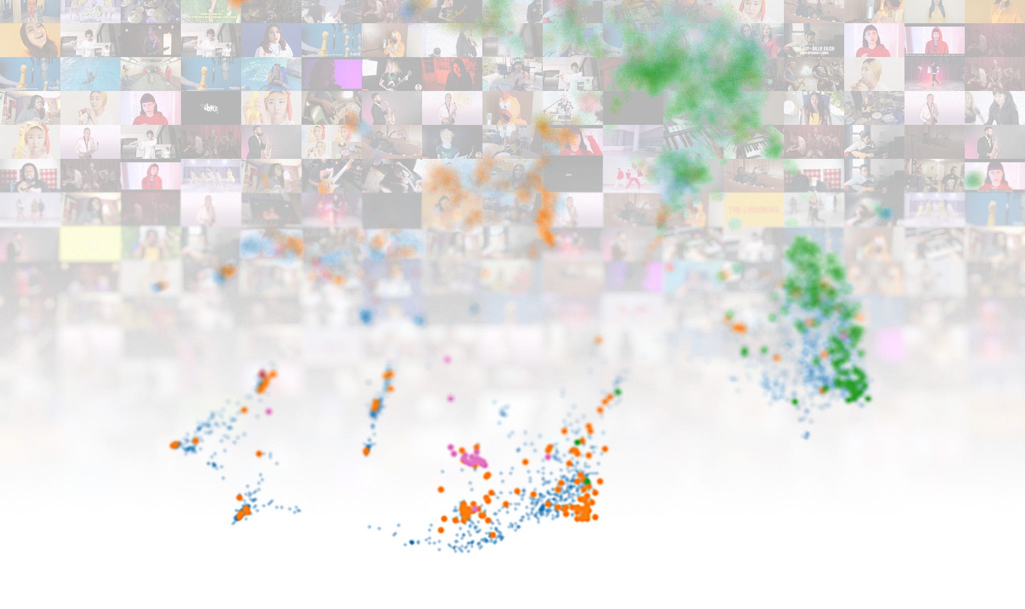
This gives us a 1280x9 + 1280 + 1280 = 14,080 dimensional vector as a fingerprint representing each video. These fingerprints can be compared with Euclidean distance to find visually similar videos. Looking at a UMAP plot overlaid with some of the ground truth labels reveals that this representation can be clustered in a way that captures the labels we are interested in:
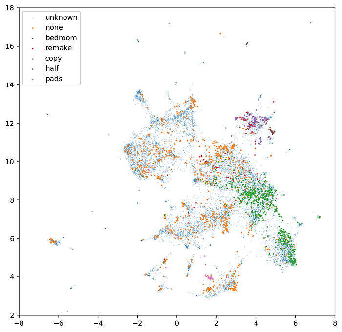
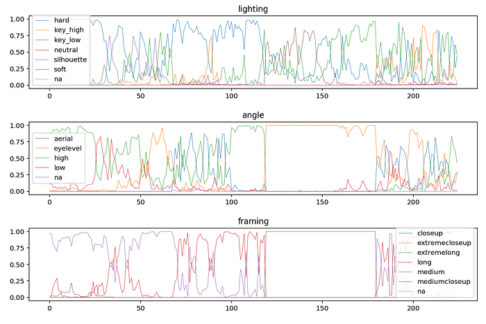
After collecting enough labels, we built a very simple dense network to predict labels from fingerprints. In production our custom classifier focused on a very small subset of our original labels: exact copies, remakes, “bedroom videos”, and MPC-style pads. Other labels were either handled by existing tools at Google or existing CinemaNet networks. Google identifies dance videos, lyric videos, instruments, etc. and CinemaNet identifies shot framing, camera angles, lighting, and texture. For the CinemaNet classifier we report both the mean value of that class across the video as well as the standard deviation, which gives some idea of whether a feature is present for the whole video or only part of it.
Conclusion
A few asides that didn’t otherwise make it into this writeup:
- librosa has a lovely example of Laplacian segmentation, a kind of structural analysis, designed to automatically identify song sections based on local similarity and recurrence. It cannot provide a dense alignment, but if we found it sooner we could have used it to make section-change proposals for manual validation — and possibly as a “confidence check” on dense alignment. Some covers that are not sonically similar to any other covers are still self-similar and structurally similar.
- Taking a similar approach as “Pattern Radio”, we tried using UMAP with HDBSCAN to cluster beats. This was one of the most promising experiments, and might be explored as a preprocessing step for other low-dimensional analysis.
- When images are resized without antialiasing, a convolutional network trained on antialiased images may perform poorly. It is preferable to rectify this during training if possible, because it can be difficult to identify during integration for production.
The biggest change we would make for next time is starting with dataset building for both visual and audio analysis from the beginning. Heuristics are tempting when doing experimental creative work, but once there is a goal it’s important to clearly define and measure progress toward that goal.
Our biggest challenge was finding a comprehensive solution that increased the quality of predicted labels and alignment across all the cover videos. Any single kind of video or cover might have a “trick” for getting better performance, but the nature and beauty of covers is that there will always be the next version that completely defies expectations.
Credits
- Technical direction and integration: Kyle McDonald
- Project management: Keira Heu-Jwyn Chang
- Initial audio analysis and annotation tool: Yotam Mann
- Initial visual similarity analysis and CinemaNet: Anton Marini
- Annotation and validation: led by Lisa Kori, with additional help from Jonathan Kawchuk, Sam Congdon, Thomas Bryans, Lu Wang, Ryo Hajika, and Chloe Desaulles.
Thanks
Massive thanks to Furkan Yesiler, Dan Ellis and Parag Mital for advising on the audio alignment algorithm. Thanks to the teams at Google Creative Lab and Plan8 for being great collaborators on this project. Especially to Jay Chen, Jonas Jongejan, Anthony Tripaldi, Raj Kuppusamy, Mathew Ray, and Ryan Burke at Google, and Rikard Lindström at Plan8. And of course, this project wouldn’t have been possible without Billie and Finneas, and all the incredible creative people who uploaded covers: thank you.
Bonus
It’s impossible to listen to thousands of covers and not pick favorites. There are plenty of covers with thousands or millions of well-deserved views. There is the 80s smooth jazz remix, Arianna Worthen’s harp cover, the lofi remix, and Pomme’s impossibly French cover, but there are many more that have flown under the radar.
- This acapella cover from Crash Vocal. Wait for the drop at 0:33.
- This “Gypsy Cover” by Jeer&Bass, who have other deceptively simple and brilliant covers (Wicked Game, Take Me Home, Country Roads).
- This country/bluegrass cover by Banjo-vie, with one of the best outro interpretations.
- This electric violin duet which also belongs in the outro hall of fame.
- This banging psytrance remix featuring Howard the Alien.
- This electric guzheng + speed painting cover.
- While tuning the alignment algorithm we fell in love with covers that are only vaguely identifiable as such, including this $1 cover on a Spongebob piano.
Footnotes
- There is a sixth category, which includes covers that do not map cleanly to this beat-for-beat paradigm, of which we only found a couple examples, including this slow jazzy cover in 3/4.
- Yes, we still used the same labels even for covers without lyrics, and for covers based on Justin Bieber’s version where he sings “gold teeth” instead of “bruises”.
- The best open source solutions for beat tracking is madmom, but due to its non-commercial use restriction we integrated the beat tracking from librosa.
- In an early iteration of this work we considered using similarity alone as a guide for the experience, but eventually decided that a user-interpretable approach was more compelling.
- For image similarity it is often more useful to use the output from the second-to-last layer as an “embedding” rather than the final classification probabilities, because the final classification probabilities lose some of the expressivity of the network’s analysis.